

Why 7.9% Returns Beat 13.9% Yields: The "Fool’s Yield" Trap
E6 - Greg Obenshain (Verdad Capital) on why BBs crush CCCs

US High yield gets often pitched as “equities with coupons”—portfolios sold on raw yields, benchmarked against stocks. But yield tells you nothing without loss risk baked in. Banks provision for expected losses in lending; high yield investors should do the same—net expected return = yield minus loss yield. Chasing CCC’s 13.9% “fool’s yield” delivers a mere 6.8%, while BBs deliver 7.9%, even surpassing the expected yield of 7.7%. A quantitative lens strips bias, controls loss risk systematically, and delivers outperformance.
Episode 6 with Greg Obenshain (Verdad Capital) shows how. What follows is the full framework.
The Fundamental Misunderstanding: Yield is Not Return
The Data Everyone Should Know
Since 1988, the relationship between starting yield and realized return in high yield tells a story that contradicts almost everything marketed to credit investors. Consider the evidence:
· High Yield Index: Average yield of 9.5%, realized return of 7.6%
· Double-B Rated: Average yield of 7.7%, realized return of 7.9%
· Single-B Rated: Average yield of 9.4%, realized return of ~7%
· Triple-C Rated: Average yield of 13.9%, realized return of 6.5%-6.8%
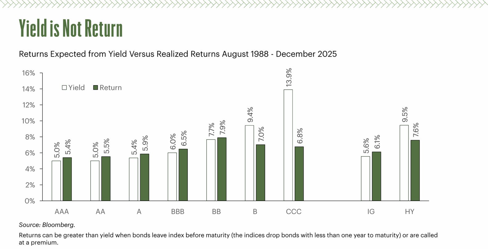
The divergence widens as credit quality deteriorates. In investment grade, yield remains a reasonable predictor of realized return—an almost 1:1 relationship. But in high yield, especially below single-B, yield functions as a ceiling, not a floor. Obenshain has termed this phenomenon “fool’s yield”—the illusion that higher yields compensates for worse fundamentals.
Investment Grade vs. High Yield: Different Economies
A critical insight separates the investment-grade experience from high yield. In IG, the yield-to-return relationship holds remarkably stable through credit cycles:
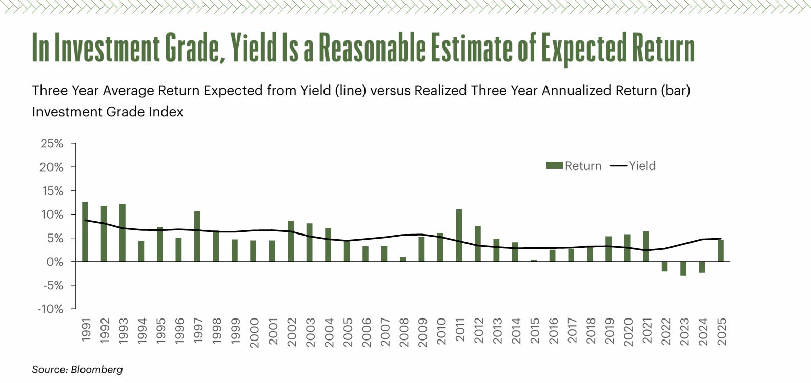
The line and bars track nearly in lockstep. This stability reflects the nature of IG credit: companies are large, diversified, and tend to experience gradual downgrades or upgrades. Defaults are rare enough that loss rates are predictable. Recent IG underperformance (2022-2024) stems partly from rising sovereign yields during the rate hiking cycle—longer duration amplified total return losses.
High yield, by contrast, exhibits violent divergence:
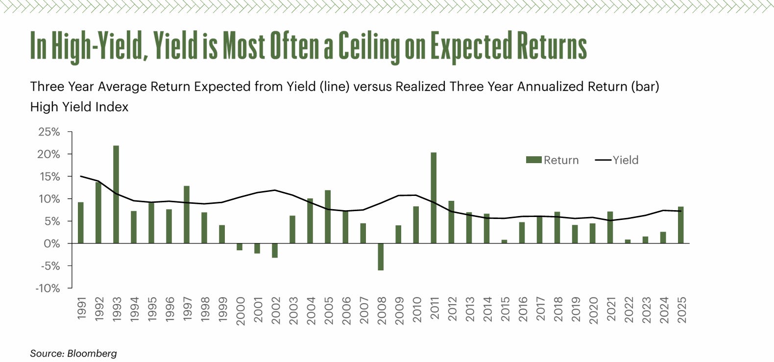
Notice the pronounced negative bars in 2002, 2008, and 2011—years when defaults spiked. The line (expected return from yield) was a terrible indicator for future performance. Investors who relied on yield as a predictor were systematically disappointed.
The asymmetry here is crucial: in IG, you can mostly trust the coupon. In HY, you cannot.
Decomposing Return: The Known and the Unknown
The Architecture of Credit Returns
Obenshain’s core insight is deceptively simple yet operationally profound: credit returns decompose into exactly two components:
1. Yield (Known): Coupon payments + pull-to-par assumption on expected cash flows. This you know upfront.
2. Loss Return (Unknown): The impact of defaults, downgrades, and spread widening. This you don’t.
Return = Yield + Loss Return
The problem is that market participants tend to treat the entire yield as “earned” return, when in fact a significant portion of it represents compensation for losses that might occur. In CCC-rated bonds, for instance, the Moody’s default rate data shows approximately 70% of issuers eventually default. If you’re buying a CCC bond at 13.9% yield and default rates are 70%, the expected return cannot be 13.9%.
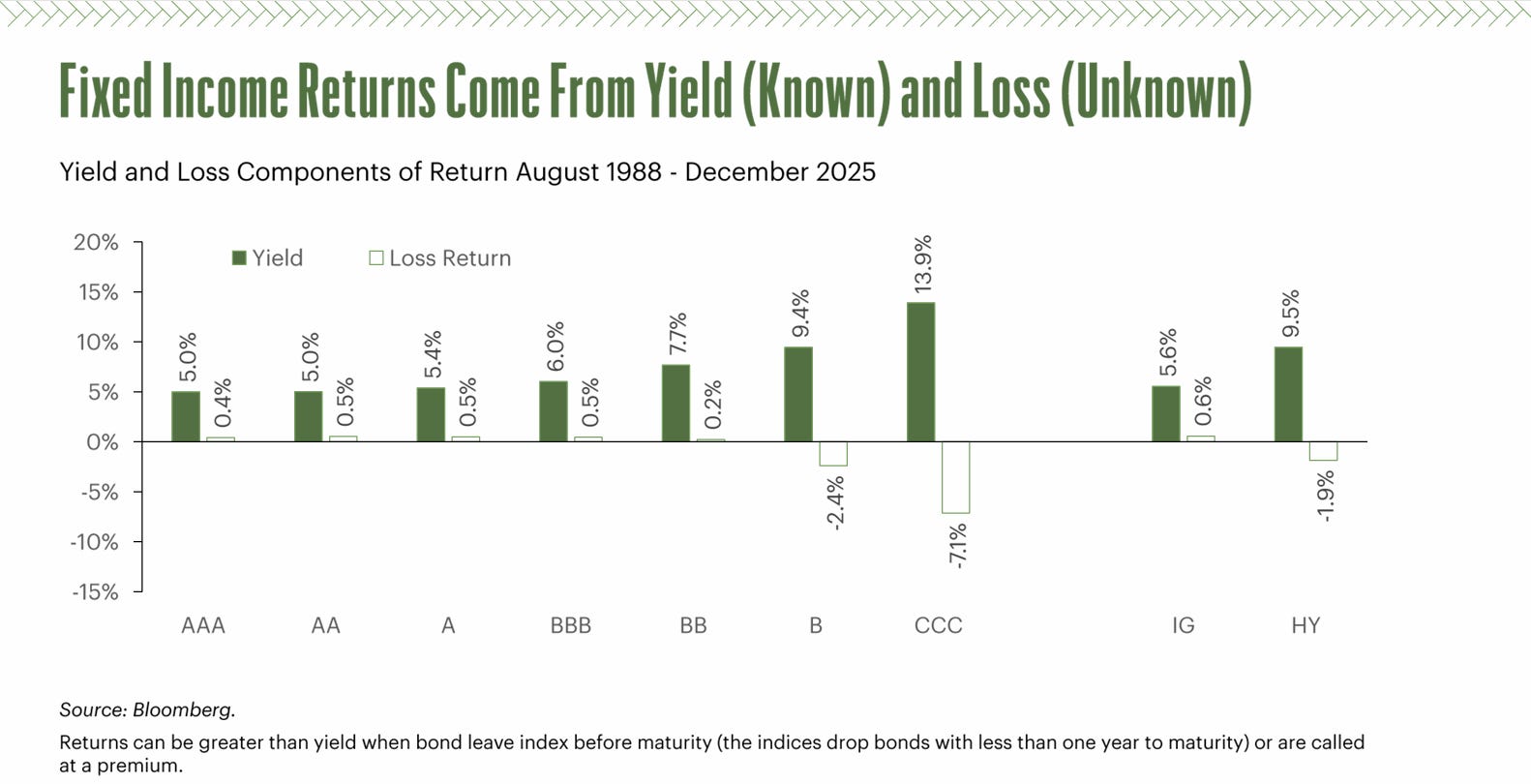
The visualization is illuminating. Notice:
· AAA through BBB: Loss return hovers between -0.5% and +0.5%, essentially near-zero noise
· BB and above in HY: Loss return remains modestly negative, ranging from -1.9% to -2.4%
· B and CCC: Loss return turns sharply negative, with CCC at -7.1%
This means a CCC investor buying at 13.9% yield can expect to realize only 6.8% actual return because 7.1% of the yield is consumed by expected losses.
The Inversion of Value in Ratings
This dynamic creates a striking inversion: the lower you go in ratings, the worse your expected return, despite ever-rising yields. This is counterintuitive because rating agencies themselves are working backward—they assign lower ratings to higher-risk issuers. But higher risk doesn’t automatically mean higher expected return in a bond; it means higher loss yield.
Obenshain makes the crucial distinction: “In credit, if you’re not shorting, your model is extremely useful for telling you what to avoid. The bottom 20-30% of the ranking is where you can really add value by not owning those bonds.”
Loss Yield as the Linchpin: Building a Predictive Framework
Why Loss Yield Matters More Than You Think
Once you accept that loss return is the critical unknown, the problem becomes tractable. Loss return, in turn, decomposes into two factors:
· Change in yield (spreads tightening or widening)
· (Credit) Duration (leverage on that change)
Duration is known in advance. So the only true unknown is: how will yields change over your investment horizon?
Instead of trying to predict a company’s future fundamentals over five years (the domain of fundamental credit analysts), quantitative analysis focuses on estimating the spread mispricing relative to fair value.
Obenshain argues this is exactly what factor models do well. If you can predict which companies’ spreads will tighten and which will widen, you’ve solved credit.
Factor Models That Actually Work in Credit
The three pillars of his factor framework are classical—value, momentum, quality—but their implementation in credit is sector-specific:
Value: Assigning an “implied rating” or fair spread to each bond based on fundamentals and market pricing. If a bond trades at BB spreads but your model thinks it deserves BB- spreads, you expect spread widening (and thus negative return). This is exactly what a fundamental analyst does, just systematized.
Quality: Heavily weighted toward rating, but also incorporating size. A striking finding: total assets is incredibly important. Larger, more established firms are less likely to default, and this advantage persists even when basic credit metrics look similar. Fallen angels (large companies that slip into HY) outperform comparable double-Bs partly because of scale and hidden strategic options.
Momentum: Here credit diverges from equities. In investment grade and BB-rated, momentum shows mean reversion: if a bond has outperformed, spreads tend to mean-revert. But in single-B and CCC, momentum becomes trend-following: if a credit is deteriorating, it tends to keep deteriorating. This means factor loadings on momentum must vary by rating—a global coefficient won’t work.
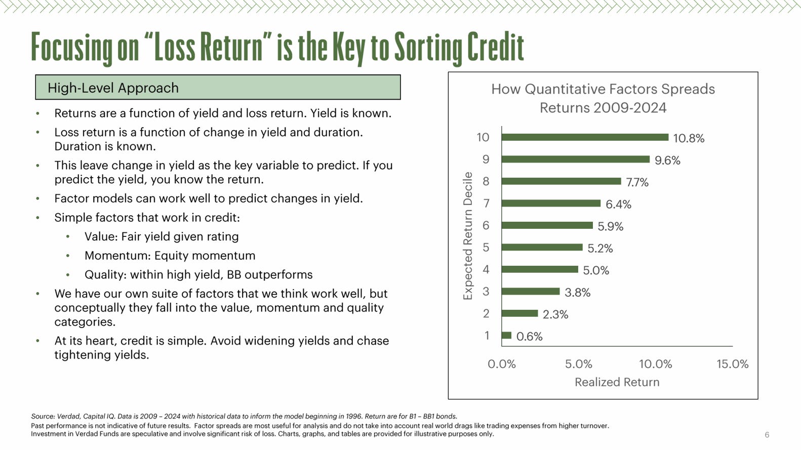
Putting It Together: The Decile Test
The proof is in performance. Obenshain’s factor model, applied to B1-BB1 bonds from 2009-2024, produced:
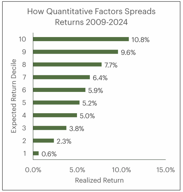
The top decile (bonds the model rated as highest expected return) realized 10.8% annualized return. The bottom decile achieved 0.6%. The spread is 10.2 percentage points—meaningful alpha.
Critically, this alpha comes less from owning the top decile than from avoiding the bottom. If you own the entire universe with equal weight, you get some baseline return. By eliminating the worst 10%, you materially improve outcomes. By actively harvesting the best 10%, you improve further. But the distribution matters: the upside tail is compressed (capped near the coupon plus modest spread tightening), while the downside tail is long and thin (defaults and distress). This is the opposite of equity factor models, where alpha is often symmetric.
The Credit as a Savings Vehicle Framework
Why High Yield Is Not Equities in Drag
One of Obenshain’s most powerful contributions is reframing how portfolios should think about credit allocation. The conventional view treats high yield as a “risk asset”—a lower-volatility alternative to equities, essentially equities in disguise. This leads institutional allocators to size credit positions based on equity risk budgets and to demand equity-like returns (8-10%+ annually).
Obenshain rejects this entirely: “I reject the premise that credit is a hybrid instrument between bonds and equities. It is its own thing.”
The evidence is in the return distribution:
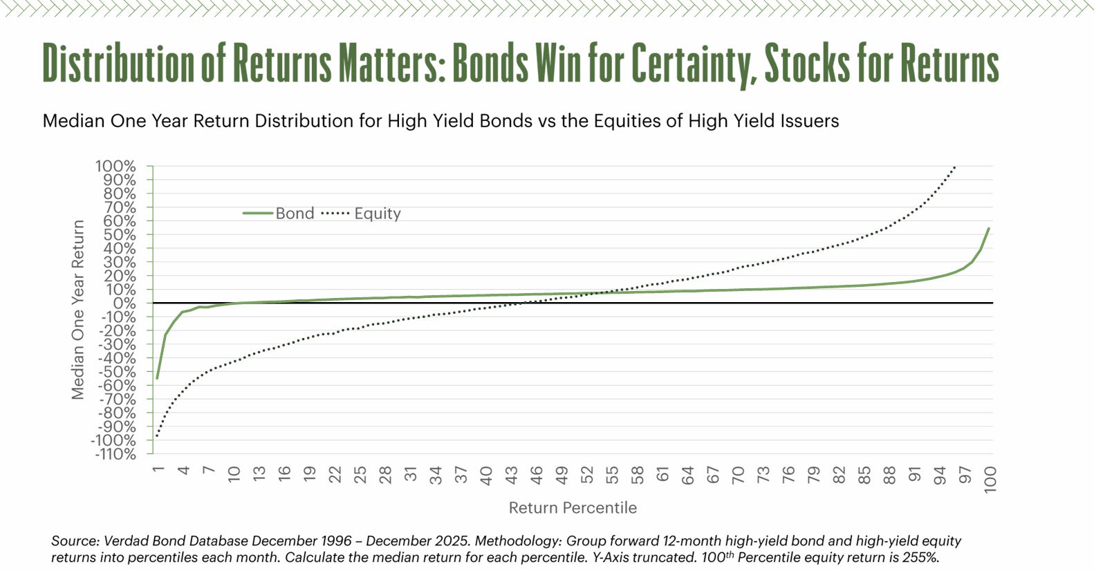
For equities, the distribution is roughly S-shaped:
· Worst percentile: ~-97%
· 25th percentile: ~-19%
· Median (50th): ~+4%
· 75th percentile: ~+32%
· Best percentile: ~+255%
For high yield bonds of the same issuers, the distribution is remarkably compressed and symmetric:
· Worst percentile: ~-55% (matching typical default recovery rates)
· 25th percentile: ~+3.3%
· Median (50th): ~+6.8%
· 75th percentile: ~+10.4%
· Best percentile: ~+54%
The bonds don’t go negative until around the 10th percentile. This is a savings vehicle characteristic: predictable, contractual, modest upside, defined downside. Equity distributions are very binary.
Who Should Own Credit, and Why
This framing has profound implications for asset allocation. Credit is appropriate for:
1. Insurance companies that must have certainty of returns
2. Endowments and pension funds with intermediate time horizons (3-5 years)
3. Individuals saving for specific near-term liabilities (tuition, house down payment)
4. Portfolios requiring downside protection without equity volatility
Credit is not appropriate for:
1. Investors who need equity-like returns (10%+ annually)
2. Long-term growth portfolios where alternatives (equities, real assets) offer better compound returns
3. Portfolios with high risk tolerance that can absorb severe drawdowns
Obenshain invests in credit for his children’s college funds specifically because he wants certainty of outcome—the bonds will likely be held to maturity, or sold without material loss, and the money will be there when tuition is due.
The expected return universe for credit is 4-8% annually for investment-grade credit and 5-10% for high yield, depending on cycle and rating. Anything above 10% annually should be flagged as either (a) outlier cycles or (b) requiring equity-like risk, which means you’re not getting the benefit of credit’s return predictability.
Market Structure: Why the Index Matters
The Secular Shift in Credit Composition
The high-yield market has undergone a structural transformation over the past 15 years that most participants don’t fully appreciate. Two metrics illustrate this clearly.
The Quality Creep:
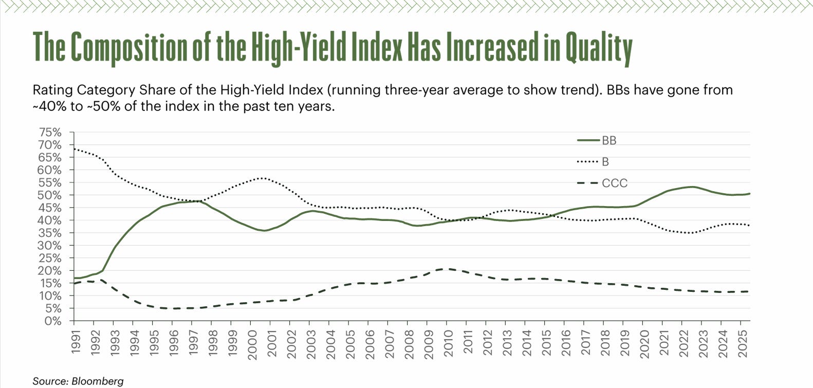
BB-rated bonds have grown from approximately 40% of the high-yield index to 50% in the past decade. Meanwhile, CCC exposure has compressed. This isn’t random; it reflects issuance patterns and the universe’s natural evolution. Many CCC companies default; many BB companies get upgraded out of HY over time.
The implication: the “average” high-yield portfolio is higher quality today than historically. This should matter for your allocation decisions. If you think the universe is riskier than it appears on the surface, you’re likely underweighting the real dynamics.
The Duration Compression:
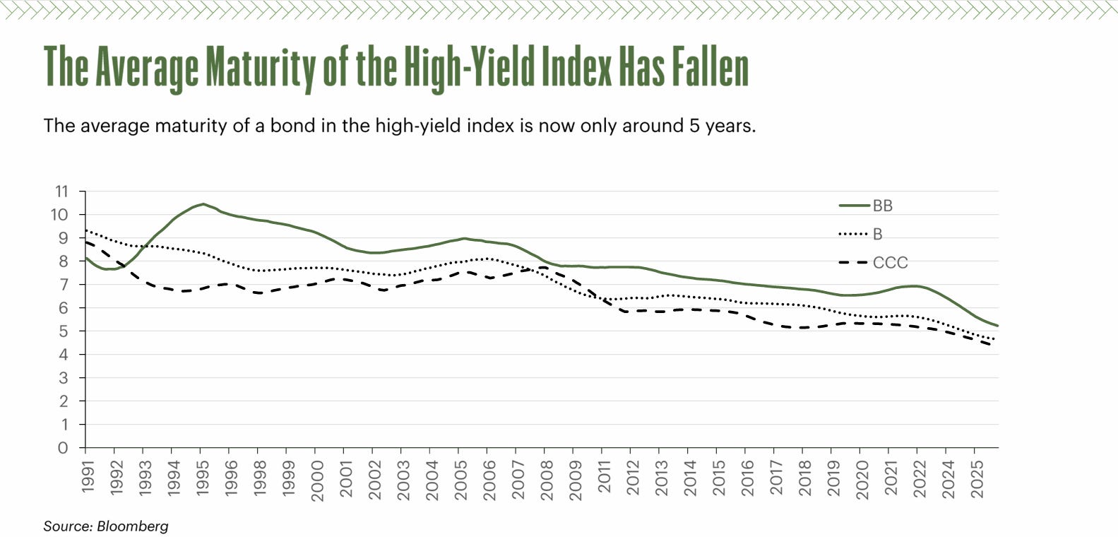
Average maturity in the HY index has fallen from peaks of 8-10 years to roughly 5 years today. This suggests that market participants are consciously trading duration risk for carry and avoiding uncompensated leverage. Obenshain notes: “If you look at the average maturity of the high-yield index across rating categories, it has been trending down toward about five years. That suggests many investors are thinking the same way: they like the yields but do not want uncompensated duration risk, especially in today’s environment.”
From a portfolio construction standpoint, this is healthy. It suggests maturity is being matched to economic horizon and that investors aren’t lever up beyond what they need.
Spread Levels as a Market Timing Signal
Spreads themselves carry predictive information about forward returns. When spreads are tight (low), expected returns compress—the model should be more conservative. When spreads are wide, expected returns expand—the model can be more constructive.
At time of writing (January 2026), spreads remain near historical lows despite recent volatility. This aligns with Obenshain’s current positioning: short duration (to minimize the leverage from modest spread widening), up in quality (to favor credits where loss yield is low), and careful in avoidance of the lowest-rated bucket.
Building the Portfolio: From Theory to Practice
The Universe Definition Problem
Obenshain starts portfolio construction with a pragmatic constraint: data quality. While investment-grade data is excellent and BB-rated data is quite good, B-rated data is “okay” and CCC data is “pretty terrible.” For this reason, his team focuses on the upper part of the high-yield universe—roughly B1 and above.
This is a feature, not a limitation. There is “plenty of money to be made lower down, but the data gets spottier—more private companies, less disclosure.” In quantitative investing, garbage in equals garbage out. It’s better to own a well-modeled, smaller universe than a poorly modeled, broader one.
Within the model, there’s a notable cliff between B1 and B2 in loss yield. Below that threshold, loss yield picks up materially, widening the gap between yield and realized return. Even within double-Bs, the dispersion is huge—some companies reliably earn their yield; others don’t. The model needs to sort within ratings, not just across them.
Duration Risk vs. Credit Risk
Obenshain generally avoids excess duration. “We want credit risk, not rate leverage,” he notes. In his framework, yield tends to maximize in the 3-5 year maturity range, then flatten. Anything beyond 5 years is mostly leverage—additional compensation for duration risk rather than credit risk.
The exception: he will take duration risk in names he “strongly likes,” because that’s leverage on a good idea. But the baseline is portfolios with “reasonably certain returns over a defined horizon, which means controlling duration.”
This philosophy aligns with the secular trends in the index (5-year average maturity today) and suggests the market is sensibly thinking through this trade-off.
The Core Ranking and Rebalancing Rule
At its core, the process is:
1. Rank every bond by expected total return (combine carry yield, expected change in yield/spread, and duration impact)
2. Apply a cyclical overlay (conservative when spreads are tight, constructive when wide)
3. Rebalance systematically, selling names that fall below the 70th percentile in the ranking
4. Concentrate buying into the top 10-20% of the ranking, especially when diversified
The key discipline is rebalancing discipline. Selling winners as they fall in the ranking—especially names that slip into the bottom quintile—is often psychologically difficult but critical. “The bottom 20-30% are the area to avoid,” and harvesting that tail is often more important than picking winners.
Sector Applications: When Standard Models Break
Why Biotech Broke Quantitative Models (And How to Fix It)
Obenshain’s team recently completed deep work on biotech equity investing, an area where standard quant models completely failed. The lessons offer insights for sector-specific credit modeling as well.
Biotech broke traditional factors because:
1. Value inverted: Most expensive companies outperformed cheapest. This is because biotech has no earnings; what looks expensive (high market cap relative to zero earnings) is actually a high-spend, high-ambition company likely to succeed.
2. Quality metrics didn’t work: Traditional quality screens (profitability, margins, ROA) all failed because the best biotech companies are spending heavily on R&D, not generating profits.
3. Momentum was noisy: Simple price momentum didn’t distinguish real progress from noise.
The solution required rebuilding factors from first principles:
· Value: Market cap relative to R&D spending (inverted from traditional metrics)
· Quality: “Specialist ownership”—whether biotech-focused funds own the name. This crowd tends to be very good at assessing probability of success and market size.
· Momentum: Clinical trial data. By building a database of trial characteristics and outcomes, they could measure whether a company’s pipeline was strengthening or weakening, independent of stock price.
The broader lesson is crucial: sectors with broken standard models are often the most attractive for differentiated analysis.
Applying This to Credit by Sector
In credit, similar logic applies. Energy credit looks very different from retail credit from a fundamental perspective:
Energy is a return-on-assets business. Reserve disclosures and production per unit of assets are exceptional sorting variables. The basic reserve section of a 10-K often tells you more than the entire business narrative.
Retail requires different metrics—you need profitability metrics (gross profit per assets, margins, earnings volatility)—because ROA isn’t the driver.
Obenshain has built both global models with many metrics and industry-specific models. Industry-specific models “add a lot of value” because they recognize that the economic drivers differ.
For a credit investor reading this: if your factor model treats all sectors the same, you’re leaving alpha on the table. The best models are industry-specific or at least have industry-specific factor loadings.
The Process Is as Important as the Model
Two Key Lessons from Quantitative Investing
Obenshain distills two crucial insights from his decade building quant strategies:
1. Quant is still a fundamental exercise. Building factors that make economic sense and actually work is hard and creative. “You’re not escaping fundamental thinking; you’re codifying it.” The best factors in credit have economic rationales—size predicts default because larger companies have more strategic flexibility; momentum varies by rating because lower-quality credits are in trend-following regimes while higher-quality credits experience mean reversion.
2. Process matters as much as the model. You need “a robust process for checking, improving, and monitoring models, with clear feedback loops and a research-plus-execution mindset embedded in the firm.” Moving to quantitative investing isn’t a project; it’s continuous improvement that never ends.
Common Mistakes in Credit Models
The most frequent errors Obenshain observes:
Over-reliance on single picks: The model’s best individual idea is often a dumb idea. The top 10-20 ideas collectively are fantastic. Judging a model on single-name picks is dangerous. You should judge it holistically.
Patching outputs instead of fixing upstream: Traders often want to override specific model picks. Instead, Obenshain pushes all fixes upstream—into data ingestion, factor construction, and model design. “It’s slow, it takes years, but once you’ve built a robust pipeline, you only need to ‘model something once’ and it keeps working with incremental refinements.”
Look-ahead bias: This classic pitfall can catch even experienced modelers. If you’re backtesting with data that wouldn’t have been available at the time of the model’s signal, you’re overfitting.
Ignoring trading costs and liquidity: Some high-alpha factors fall apart once you account for the bid-ask spread and market impact of trading the signal. Always model with realistic trading costs.
Risk Management: Volatility is Not the Only Risk
Beyond Standard Deviation
Obenshain notes that “rating and duration explain a large fraction” of credit portfolio risk. Your overall risk profile is “heavily driven by your average rating and average duration. You can trade off between them—sometimes higher credit risk, sometimes more duration risk in higher quality—but those two dimensions largely define your risk profile.”
This is both more restrictive and more liberating than modern portfolio theory suggests. More restrictive because it means the two main levers are clear—you’re not discovering some hidden correlation structure that revolutionizes risk. More liberating because it means you can simplify your risk modeling.
Correlations matter in credit too, especially in stress when everything compresses. But they matter less for long-only credit than for long/short equities because:
· Short opportunities are limited (lower-rated bonds offer asymmetric risk)
· The return distribution doesn’t go deeply negative until around the 10th percentile
· Most gains come from being positioned in the right quality/duration band
Once you’ve set your average rating and average duration targets, Obenshain focuses on selecting “the best expected returns within those constraints” rather than spending enormous energy on correlation matrices.
Corporate Actions and Qualitative Risk
One often-overlooked risk factor in credit is corporate action risk. Liability management exercises, covenant-stripping deals, refinancings, and M&A can create sudden repricing. These require ongoing attention.
However, Obenshain’s analysis shows a striking pattern: “On average, corporate actions are a net positive in higher quality credit.” The loss-return breakdown by rating shows that investment grade and BB-rated bonds realize slightly positive loss return—you actually earn more than the starting yield would suggest. This is because calls at par, tenders at premiums, and takeouts above par offset baseline defaults.
The implication: “Don’t try to make your return on bad companies. Focus on decent credits where corporate actions are more likely to work in your favor.”
This is exactly backward from how many traders approach credit. They hunt for distressed situations and downgrades, assuming volatility creates opportunity. Obenshain’s evidence suggests the opposite—better risk-adjusted returns come from high-quality names where the structural likelihood of positive corporate actions is highest.
The Current Environment and Forward Guidance
Today’s Setup in Context
At the time of writing (Q1 2026), Obenshain’s framework points to a specific positioning:
Tight spreads signal modest widening over 3-6 month horizons, projecting price losses
Index quality elevated (BBs ~50%, CCCs down)—trend continues as liquidity dries up for low ratings
Short duration imperative: “Collect yield but don’t lever losses with long duration”
Avoid losers ruthlessly—”they have so much negative convexity embedded” (B2s/CCCs underweight)
Sell discipline: Bonds below 70th percentile ranking get cut; bottom 20-30% avoided entirely
This is deliberately cautious but not bearish. Obenshain emphasizes that he “doesn’t try to predict market timing on an absolute basis.” Rather, this is a relative statement: given tight spreads, the expected risk/reward has shifted.
The Baseline Remains Intact
What hasn’t changed is the long-term framework. The best returns in credit still come from:
· Avoiding the worst-quality quintile
· Focusing on reasonable credit quality (BB1 and above)
· Matching duration to economic horizon
· Being diversified enough to capture what the model does well
· Rebalancing discipline
If and when spreads widen materially—say, to 400-500 bps in high yield versus 350 today—the model will turn more constructive. But that’s a future state, not today’s reality.
Verdad Capital’s Research and Philosophy
Building an Intellectual Foundation
Beyond the specific factor work and portfolio application, Obenshain and Verdad Capital maintain a published research program aimed at the thinking investor. Their weekly Monday-morning research email (archived at Verdadcap.com) covers credit markets, but also biotech equity, Japanese equities, and other topics—always grounded in serious quantitative and fundamental work.
Obenshain credits this research publication with keeping the firm intellectually honest. “We have a large research library and a weekly Monday-morning research email we’ve been sending out for about 10 years. The entire archive is on the website.”
For credit professionals looking to deepen their understanding, this archive is invaluable. The recurring themes—return decomposition, factor model construction, sector-specific analysis, and risk management—provide a continuous education in systematic credit investing.
The Integration of Equity and Credit
Finally, Verdad Capital runs both equity and credit strategies with an integrated quant team. This cross-asset perspective is rare and valuable. Many insights from equity factor modeling apply to credit (quality, momentum, valuation), but credit offers unique opportunities because:
· The return distribution is more predictable
· The downside tail is capped (known loss rates)
· Long-only strategies can still be powerful (no need for shorts)
This integration is visible in their biotech work, where clinical trial data (a fundamental driver of equity returns in small-cap biotech) becomes a factor in their equity modeling. In credit, similar integration happens—corporate actions, leverage ratios, and fundamental quality metrics serve both disciplines.
Conclusion: A Framework for the Thinking Investor
Credit professionals operate under pressure to deliver consistent returns in an asset class that is structurally unpredictable. This paradox—contractual obligations that can be broken, yields that promise but don’t deliver, comforting simplicity hiding complexity—is what makes credit interesting and difficult.
Obenshain’s work offers a path through this maze: stop treating credit as “equities in a tuxedo,” accept its nature as a savings vehicle with defined risk and capped upside, and build systematic processes that correctly distinguish genuine alpha from illusion.
The core insights are:
1. Yield is not return. Especially in lower-rated credit, yields overstate expected returns because they embed loss assumptions.
2. Loss yield is the key. Once you decompose return into known (carry) and unknown (loss), the problem becomes tractable. Loss yield depends on spread changes and duration. Spreads can be modeled probabilistically.
3. Quality matters more than rating. Within any rating, there’s huge dispersion. Larger companies, with better fundamentals and more strategic options, earn their yield. Smaller, more leveraged companies often don’t.
4. Process beats predictions. Invest in data quality, factor construction, and rebalancing discipline. Resist the temptation to override the model on single picks.
5. Avoid losers, don’t worship winners. The edge in credit comes from not owning what will deteriorate, not from perfectly timing what will rally.
6. Match structure to objective. If you want certainty, credit works beautifully. If you want equity-like returns, you’re asking credit to solve the wrong problem. Allocate accordingly.
For a credit professional reading this in early 2026, the environment suggests staying in high-quality (BB1 and above), controlling duration, and being patient. Yields remain attractive but not exceptional. The real opportunity lies in having the discipline to maintain quality and duration discipline while avoiding the worst-rated quintile—a process that will outlast any single market cycle.
Listen to the full episode for Gregs’s take on Quantitative Credit.
This article is based on Episode 6 of Fixed + Floating, featuring Greg Obenshein of Verdad Capital. The views expressed are those of the speakers and do not constitute investment advice. For more information on Greg’s research, please visit https://verdadcap.com/.
Fixed + Floating is the premier podcast for institutional investors and finance professionals exploring the forces shaping global credit markets. Hosted by Portfolio Manager Josef Pschorn, the show features conversations with leading voices from investing, research, and academia. We analyze the technical mechanics of High Yield, Private Debt, and Distressed Situations—from covenant evolution and liability management to macro policy impacts on credit cycles—providing forensic depth for the global fixed-income community.
Support Material:
Obenshain, Greg. “Fool’s Yield.” Verdad Capital Research. 2019.
Obenshain, Greg. “Yield Is Not Return.” Verdad Capital Research. 2024.
Verdad Capital. “Base Rates in Fixed Income.” Research publication. January 2026.
Hey, great read as always, this analysis clearly demonstrates how a robust quantitative framework is essential to avoid the 'fool’s yeild' trap and accurately project net expected returns in high-yield markets.